It’s common practice in the tech sector today to excite investors, job applicants, and news organizations by using the term “machine learning.” As the term grew in popularity in the latter half of the 2010s, its definition slid from academic to cultural, from rigid to soft. Where previously only machine learning engineers used the term, now most individuals who engage with current news need to at least understand vaguely what the term means. The result is a blurring of machine learning’s commonly understood meaning. This transition isn’t necessarily bad—it’s a natural result of an academic term becoming a common conversation topic—but a soft definition does create more space for miscommunication, especially when the new soft definition is reintegrated into academia through a new generation of students and researchers. Maintaining a clear definition of machine learning is important for ensuring everyone understands what everyone else means when they use the phrase.

Linguistic Approaches to Definitions

In linguistics, there are two perspectives on how to investigate language features. The older of the two is prescriptivism, in which linguists look at a language’s agreed-upon definitions and conventions, and use those to judge peoples’ language usage as either right or wrong. The more contemporary of the two is called descriptivism. Descriptivist linguists seek to describe how language is used by people who speak it, not how speakers claim it should be used. Often how we assert we should speak and how we actually speak don’t align perfectly.

An available case of this disagreement is how the two groups treat infinitive-splitting in English. Prescriptivist English grammarians dictate that nobody should ever split an infinitive (”I want to accurately meet your specification”), opting to bring adverbs outside of the infinitive (”I want to meet your specification accurately”). Descriptive English syntacticians observe that English speakers naturally split infinitives in everyday speech despite their being taught not to do so. For this reason, descriptive syntacticians accept infinitive-splitting as part of natural English grammar. Descriptive linguistics dominates the higher-academic field in part because it’s able to capture the way languages evolve over time. Prescriptive linguists slowly drift apart from how language is presently used until they are describing a language which no longer exists, or until a new set of language rules are established and they begin the slow desynchronization process again.

Descriptive and prescriptive linguists also have different approaches to constructing definitions. To the prescriptive linguist, definitions exist in language a priori, and do not change over time. When a new term is created, its definition is set in stone. To the descriptive linguist, a definition is entirely based on how the term is used. This is how Merriam-Webster came to define “literally” as “in effect : virtually” in 2011. Since the word was commonly used to as emphasis at the time, its descriptive definition changed to account for that usage.

Descriptive definitions are better at capturing a term’s common meaning, and at introducing people unfamiliar with the term to how they should expect to see it used. Still, there is benefit to the prescriptive perspective. Prescriptive definitions can to be simpler than descriptive definitions, because they don’t have to account for the wide smear of uses a word acquires as it slowly evolves. Prescriptive definitions are used in academic and professional settings because a fixed definition clarifies discussion of complex subjects.

A descriptive definition for machine learning, one which captures all of the term’s myriad uses, wouldn’t clarify the now fuzzy definition at all. Rather, such a definition would encode the vagueness of the current term’s usage. What we’re looking for in a new definition of machine learning, then, is a compromise between prescriptive and descriptive definitions, selecting for a certain category of usage to describe. To figure out what uses to consider, we can look back at why the current term is so mired: non-technical references to “machine learning” lead people to misunderstanding its real-world meaning. Analyzing the commonalities in how machine learning engineers use the term “machine learning” can give us a specific descriptive definition of machine learning separate from its popular usage.

Comparing Types of Machine Learning Algorithms

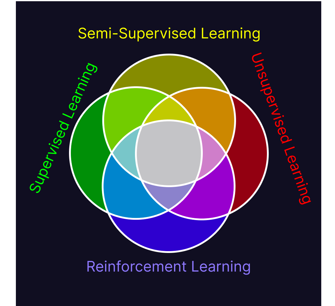
There are four ways “machine learning” is used by machine learning engineers. The four machine learning paradigms are supervised, unsupervised, semi-supervised, and reinforcement learning. Since these exhaustively cover all algorithms understood to be machine learning today, a definition which characterizes all four will necessarily be one which covers all current machine learning algorithms. The shared traits between these paradigms specify a definition which describes all of them.

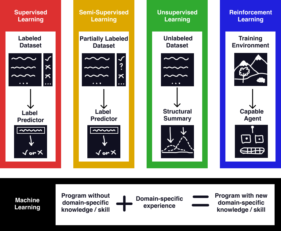
Supervised learning algorithms are provided a dataset of individual data points, each with a labeled target attribute. They use that input to learn associations between the target attribute and the rest of the data points’ attributes. Once done learning from the dataset, those associations are deployed to predict labels for novel unlabeled data. Examples of supervised learning algorithms are polynomial regression, naive-bayes classifiers, and support-vector machines. Supervised learning is by far the most common class of machine learning algorithms, since it can be used as an automation tool for human tasks. Rather than having a human identify pictures of birds, a supervised learning method can be trained on human-labeled photos of birds to identify them accurately, obviating the original labeler’s job. It’s incredibly easy to test supervised learning algorithms by checking their predictions against new labeled data, verifying their efficacy.

Unsupervised learning algorithms learn about a dataset without predicting a specific target attribute of the data. They don’t have a target to learn about, so the variety of unsupervised learning techniques are broader than supervised learning. Unsupervised learning can model what values are expected in the dataset (as in anomaly detection), it can find distinct clusters in the data (gaussian-mixture-models, and latent Dirichlet allocation), and it can find correlations between different attributes of their datapoints (ex. primary component analysis). Similar to classical statistics, unsupervised learning is useful in gaining insight about a dataset.

Semi-supervised learning algorithms are essentially mixes of supervised and unsupervised learning algorithms, in which some of the data is labeled and others are not. The access to unlabeled data can help the program train more accurately on the smaller labeled dataset it is afforded, in using the relations learned in the large dataset to assist predictions in the small dataset. When acquiring labeled data is difficult, semi-supervised learning techniques can be the difference between a working model and a broken one.

Reinforcement learning algorithms are the most unique of the four, and are structured around autonomous agents maximizing their reward within an environment. These do not train on datasets, but rather interact with an environment and are given rewards for completing desired goals. One example of reinforcement learning is a mechanical arm and camera attempting to grab an object. The optimal way to grab an object is difficult to express to the computer, but it can learn on its own via trial and error, with reward being given upon a successful grab. Reinforcement algorithms tend to be uncommon, as they require spontaneous feedback to novel solutions from the program, which may need to be evaluated by hand on a case-to-case basis, or in an environment which needs to be manually reset. Still, in some scenarios, they are by far the most effective method, especially if an automated test-environment, or “teacher” can be encoded. In fact, this is what occurs in generative adversarial networks (GANs), which use a powerful “discriminator” supervised algorithm to train a “generator” reinforcement algorithm.

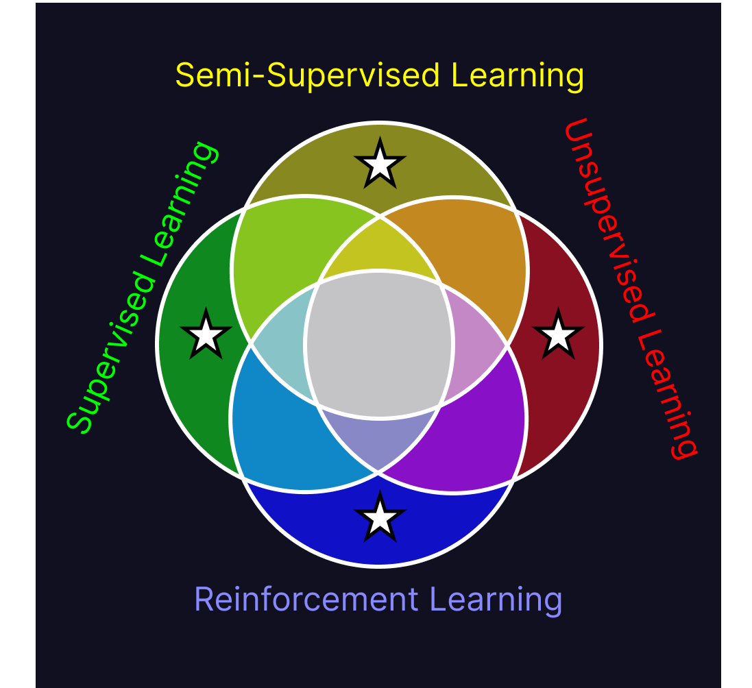
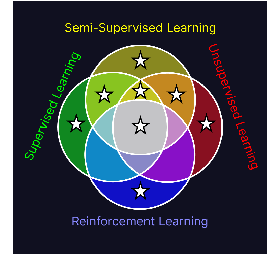
Now that we know what each of these algorithms are, we can start looking at commonalities between them. Finding the shared traits of all four paradigms at once is difficult to do, but a much easier task is iteratively combining similar paradigms until we reach the center of the Venn diagram. Doing so lets us compare just two groups of algorithms at a time, rather than all the algorithms at once. I’ve put stars in each of the sections of the diagram we’ve discussed so far.

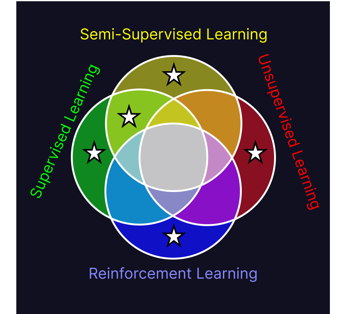
Looking at the commonalities between supervised and semi-supervised learning, both attempt to predict a target value based on the values of their input data. Supervised learning does so based only on the relations it’s learned between individual data and their associated target value, whereas semi-supervised learning also explicitly learns about internal structure in the dataset as a whole and how that can be used to help predict the target value.

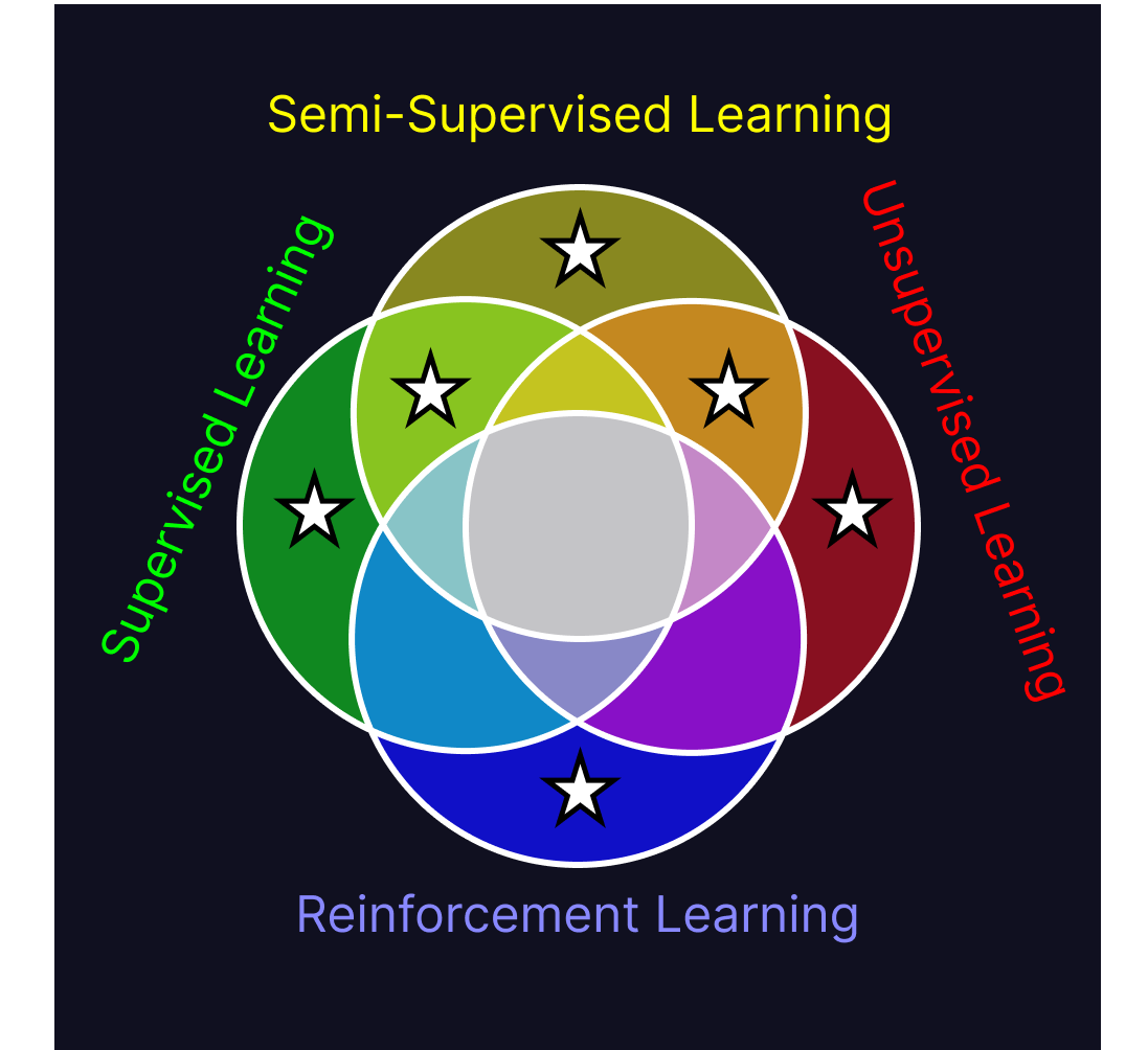
Semi-supervised learning and unsupervised learning both learn about the structure of their datasets. Semi-supervised learning does so in order to find insight into a target value, whereas unsupervised learning does so for the value that structural knowledge of the dataset provides on its own. While semi-supervised learning is deployed for the purpose of predicting a target attribute, unsupervised learning creates new attributes of the data (ex. what cluster is this datapoint), and can be deployed to assign new data points those novel attributes.

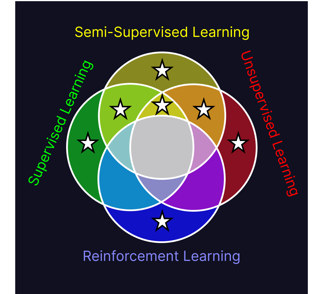
Supervised learning, semi-supervised learning and unsupervised learning all train variables using a pre-defined structure and learning method on existing datasets to produce models. In all of these techniques, those models then evaluate novel data similar to their training data. All of them have this structure: Set up model structure, train model on data, deploy model on novel data.

The difference between the gold segment, (the intersection of supervised learning, semi-supervised learning, and unsupervised learning), and reinforcement learning, is in their training method. The triplet here all have the commonality of learning information off of a dataset, whereas reinforcement learning trains within an interactive environment.

Reinforcement learning can be likened to supervised learning in that it uses prescribed feedback on its judgements to train its model, but it’s also similar to unsupervised learning in that it has to explore structure within the environment in order to figure out what sequence of events are required to trigger a reward. Though these different approaches to training are hard to reconcile into a single model, they have commonalities. All of these models use information from their training environment to perform a task better than they could prior to being exposed to that environment. Across all of the subfields of machine learning, a machine learning program is one which gains new abilities through exposure to its working environment.

Critiques of this Definition

Are Perpetual Learning Algorithms Machine Learning?

This definition is broad, and people could protest that it does not capture specific traits of the machine learning field. One thing that almost all machine learning algorithms have in common is a training period and a separate deployment period. This is the case because most algorithms are much more time consuming to train than to deploy, and so if the model can run in a deployment environment without simultaneously training it tends to be faster than if it remained training. This is why most machine learning models today are incapable of learning beyond their training stage—the resultant models have no learning capacity, but rather are the result of a learning period. Still, the average machine learning engineer wouldn’t say that perpetual learning algorithms fall outside of machine learning’s domain.

Is Caching Machine Learning?

Another contention could be that this definition covers algorithms which are not machine learning. Pure functions are programs which take input and produce a deterministic output. In other words, each specific input only has one output when used in that function, and that output never changes. Multiple outputs can have the same input, but each input always maps to the same output whenever the function is called with it.

For example, this pure function takes the square root of its input number, and every time I put in 100 it will always output 10.

1
2
3

# Exponentiate a number to the 0.5th power to take its square root
def square_root(number):
  return number ** 0.5

This impure function returns a random number between 0 and the input number. If I put in the number 15 three times, we’ll see three completely different results.

1
2
3
4

# Multiply the number by a new random value each function call
# random() returns a random decimal number between 0 and 1
def random_number(number):
  return number * random()

Caching algorithms are wrapper algorithms which augment pure functions. What caching algorithms do is keep track of recently used input-output pairs to the function. When the function is called with a recently used input, the caching algorithm intercepts the call and returns the stored value, stopping the function from re-calculating it. For process intensive functions with few inputs, these caching algorithms can increase their speed drastically. In some sense, these caching algorithms fall under the definition of machine learning described above. In being exposed to their working environment (the function being called with test data), they improve the function’s operation speed. A caching algorithm which has never been exposed to any function calls will definitively not add any optimization to the first call it handles, but as it runs it becomes more effective until it reaches an upper limit on its ability to preempt what inputs will occur next.

Though some would describe caching as machine learning, most people I surveyed consider it too dissimilar from conventional machine learning. In interviewing colleagues about why they felt it was or wasn’t machine learning, all of the dissenters agreed on the reason they thought it wasn’t machine learning: caching does not provide enough new un-encoded functionality to qualify as machine learning. In this case, they actually agreed with my definition, and contended that caching algorithms do not acquire new skills, but rather use a pre-encoded method to accelerate pre-encoded functionality. In this sense, the definition we came to proves to be more robust, in that it aides people in clearly describing why a controversial model is or isn’t machine learning to them. A good descriptive definition gives people grounds to justify their gut instinct on whether something is or is not part of that definition.

How this Definition Helps Everyone

By striking a balance between descriptive and prescriptive definitions, it’s now clear what machine learning is from the perspective of machine learning engineers. This doesn’t mean that every reference to machine learning will fall under this definition; as mentioned at the start of this article, the term will get misused by people who have a vague understanding of the term. However, with the knowledge from this article, it’s easier to recognize when the term is being used carelessly. As more people learn the technical meaning of machine learning the public discourse surrounding it will become more precise and easier to understand for everyone involved. It’s helpful when studying a subject to set the bounds on where that subject starts and ends.
Rigorous definitions help in defining what is on the table for discussion, which is especially valuable when looking for novel approaches to difficult pr oblems. For the past ten years, the most groundbreaking computer science advancements have been in machine learning. Those achievements often¹ (though not always²) were the result of novel perspective shifts on algorithm design. Finding novel approaches within the bounds of machine learning means looking at novel ways This concrete definition of what machine learning is helps computer scientists explore the field’s unreached edges.

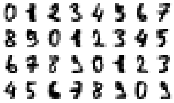
I have a machine learning model that can analyze what number is depicted in a picture.

What number is this?

3

What number is this?

8

What about this?

7

Extrapolation in Supervised Machine Learning

Supervised machine learning methods are a subset of machine learning which, given a datapoint composed of known attributes, predict an unknown target attribute. They achieve this task by training their predictive model on a set of datapoints with pre-labeled target values, finding patterns of relation between the known traits and the target trait.The model’s predictions are ‘supervised’ by the training algorithm in that they are judged against the true target labels in the training dataset. Supervised methods are the most commonly used machine learning tactic today, as they are especially effective at automating the prediction of complex relations between known inputs and outputs, a skill which allows programmers to automate human evaluations of data. These models, however, lack a subtle but crucial trait humans use without realizing in prediction. In trusting them to evaluate data without oversight, programmers open ourselves up to vulnerabilities which would never occur in the human evaluations these systems mimic.

When a human is given a data evaluation task, they effortlessly recognize when the data they are given is abnormal. In an effective task structure, if the abnormality seems relevant to the evaluation, the data is marked as unable-to-eval and/or escalated to someone with more knowledge. As with most computer programs, supervised learning methods are content to take in clearly anomalous data and indiscriminately process it.

In some respects the capacity to extrapolate is desired! In traditionally written code, more general programs are usually considered more refined for two reasons: (1) they reduce the amount of new code which may need to be written in the future, and (2) their design grasps a deeper abstracted general problem underlying the more immediate problem at hand. The second is clearly inapplicable to supervised learning methods, as their capacity to function on new data is not an abstraction away from the immediate problem, but rather an application of the current heuristics to a new domain. The first is true only on the condition that the model extrapolates outside its training set accurately… which may be true, but may as well not be. A programmer has no way to know if their model extrapolates well into a new domain without hand-labeling data from that domain and evaluating the model against it. Without a way to isolate and manually label the anomalous input from the sea of data fed into the model for judgement, we risk extrapolating into a domain our model is completely unequipped to judge. Worst of all, we wouldn’t even know that our model performed an erroneous judgement, because to it the inputs’ differences from the training set are completely ignored.

Luckily there is a way for our model to notice strange input: Anomaly Detection. Anomaly detection algorithms are a class of machine learning focused on identifying anomalous data. There are many ways to perform this task, with some being more suited to particular situations than others. Regardless of which anomaly detection algorithm is used, incorporating anomaly detection into a supervised learning model is easy! Just train an anomaly detection algorithm on the same data your model is trained on, and if the detector goes off on a production datapoint return an error instead of an evaluation. This allows whatever system the model is interacting with to handle the anomalous data whatever way it wants, storing it for human inspection, skipping further processing on the data in the same pipeline, etc.

A Solution In Practice

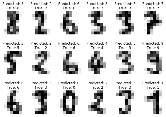
Let’s say I wrote a machine learning program to recognize images of handwritten numbers. It’s intended to be used in reading ID codes on scanned library stack cards. It’s 98% accurate on data it’s never seen before, which is good! Good enough to deploy at least.

A few weeks after I deployed it one of the librarian assistants came to me saying that the model started outputting numbers totally irrelevant from the numbers on the cards. This could have been going on for a while, since they only noticed after searching for some of the IDs they knew were in the prior day’s stack and not finding them in the system.

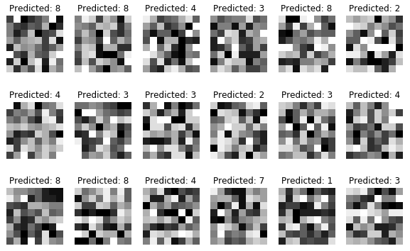
Why? After a few hours of scrutinizing and testing my model, no bugs showed… until I checked the input data. Evidently the scanner’s backlight broke, and the camera was boosting the contrast on nearly-black document to try and get a good picture, resulting in pure noise.

My model took in the data and happily spit out judgements as to what number it most associated with the noise. While we sought a replacement bulb for the scanner, I wrote some code to ensure that the model wouldn’t overconfidently judge data it didn’t fully understand again.

1
2
3
4
5
6
7
8
9
10
11
12
13
14
15
16
17
18
19
20
21

from sklearn.neighbors import LocalOutlierFactor

# Train outlier model on X_train dataset
outlier_model = LocalOutlierFactor(novelty=True)
outlier_model.fit(X_train.reshape((len(X_train), 64)))

def judge_digit(data):
  # get probabilities of each category for each picture in data
  probs = model.predict(np.expand_dims(data, axis=3))
  # get category with max probability for each
  preds = np.argmax(probs, axis=1)

  # predict which data are anomalies
  anomalies = outlier_model.predict(data.reshape(len(data), 64))

  # Set all anomalous predictions to -1
  for i in range(len(preds)):
      if anomalies[i] == -1:
          preds[i] = -1

  return preds

The solution was relatively simple! I ran an out-of-the-box implementation of the Local Outlier Factor algorithm, which is a density estimator, on the data input. I wrote a composite function which ran the density estimator on the data, and, when an outlier was detected, returned -1 rather than an evaluation from 0 to 9. This captures testing data that are clearly different from the training set (such as random data, significantly darker or lighter than normal data, and data that’s been offset from the center of the frame) while letting through data that generally seems similar to the input data. The Local Outlier Factor algorithm may not be the best algorithm for every case, but it was a good one for this particular task. Any method of producing a predictive model that judges whether a new datapoint is inside or outside the training domain will function to produce the desired capability in a composite model.

It is important to remember that the Local Outlier Factor model’s goal is not directly to guess which data the classifier will misclassify, but rather to guess which data are different from the input set. It may be true that an entire class of data (like washed out numbers) are classified correctly by the model, but in that case it is still valuable for the programmer to be alerted when these new data show up so that they can be hand-labeled and added to the model’s training set on a successive version. Re-training the supervised learning model explicitly on data which was rejected as an outlier results in the model’s domain growing with a cautious purposefulness that lends it a much greater reliability in practice. It enables the programmer to judiciously label data which will increase the model’s domain, and not waste time hand-labeling data which does not improve the model because it is situated in a domain the model already understands.

A reasonable question could be: why did I have to add the unsupervised method into my supervised learning paradigm? Couldn’t I have added an extra label, -1, to my supervised model’s category list, and provided labeled noise as part of the training data? At first glance it seems to be a simpler solution than adding an entire other learning model. There are a few reasons why this would harm the supervised model’s overall accuracy. For one, it would require us to know what the outliers will look like prior to our training the model, when the point of this task is that we want to identify data we didn’t expect. We would have to know what we didn’t expect to see in the input prior to seeing it. For another, we would have to balance the amount of outlier input we provide the supervised model, so as to not bias the model’s expectation that any given datapoint is an outlier. My categorical model (a one layer convolutional neural network), were it to be trained on too many outliers, would expect a new datapoint to be an outlier, and would require strong correlations between the new datapoint and another category to outweigh that prior bias. By using an unsupervised model for outlier detection, we minimize the effect that this addition has on the already developed predictive model that it assists.

Don’t Ignore This Advice!

This may seem like a suggestion, but domain modeling is an inexpensive addition to most machine learning programs that increases their accuracy and longevity. It’s also a good use of resources for improving a model which appears to be promising, since it can be used to collect optimal additional training data. Extrapolation can lead to systemic error that often goes unnoticed for long stretches of time, which, depending on how important your model is, can cause serious harm. The addition of even a simple out-of-the-box domain modeler mitigates the most egregious cases of extrapolation, and putting in the effort to implement a more nuanced domain modeler will catch more fine-grained cases of extrapolation.

Part One: What are Hyperparameters?

Figure A

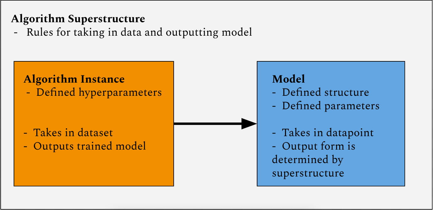
The term ‘machine learning algorithm’ is ambiguous. The component of machine learning that the public interacts with most frequently is the machine learning model, which takes data and processes it to produce an actionable result. The youtube recommendation algorithm is a machine learning model which takes in data about a user as well as data about videos on the site and recommends the user videos that optimize for sustained watch-time. Programmers are introduced to machine learning from the other end. Computer science courses introduce students first to machine learning algorithm superstructures: the steps for generating and optimizing the parameters of a model. Each algorithm superstructure also defines the format of its model, i.e. what its inputs, outputs, and intermediate structures can look like. Typically a machine learning algorithm superstructure provides some amount of flexibility in its output model structure. Between the two is the algorithm instance, which is an individual invocation of the superstructure with a set of hyperparameters that define a rigid form for the model’s structure within the broader space allowed by the superstructure. The instance is executed on a computer and trains its model’s parameters to be optimal over a provided training dataset. If a given machine learning model is a bicycle, the algorithm instance which produces it is the bicycle factory which produced it, and the model superstructure is a design document for factories that produce bicycles.

Hyperparameters exist at an interesting location within this taxonomy, because while choosing the right values for them is very important to generating an effective model for a given dataset, they cannot be adjusted during the model training process, since they determine the shape of the model. They must be defined before the expensive training process is executed.

Part Two: A Case Study in Hyperparameters

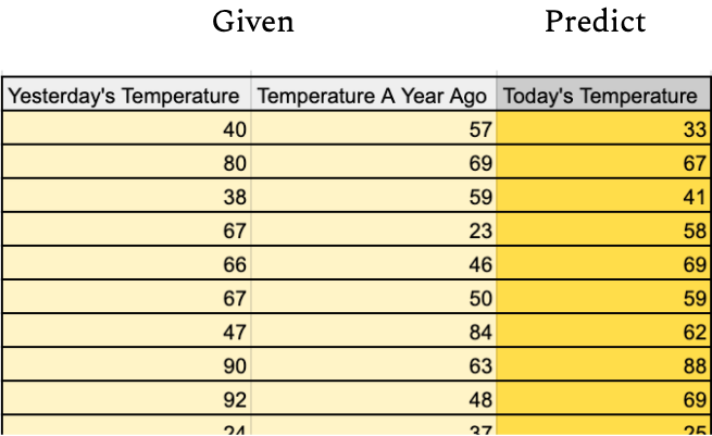
Regression algorithms are a subset of machine learning algorithm superstructures which, given a set of input values and their corresponding output values, generates a model to map those inputs to their outputs¹ (Figure B). Figure B

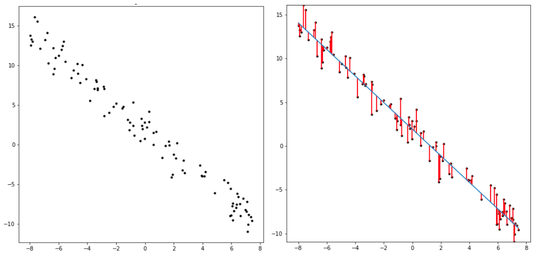
Linear regression is a simple example of this type of algorithm. It generates a line² that most closely fits a set of datapoints. The way it measures closeness between the line and the dataset is the difference between the line’s predicted y value (f(x)) for a given datapoint’s x coordinate, and the datapoint’s actual y coordinate. It optimizes two parameters: the x-intercept of the line (p_0) and the line’s slope (p_1), which are used in the relation defining the line: f(x) = p_1*x + p_0 . The linear regression algorithm finds the values of p_0 and p_1 which minimize the difference between f(x) and y for all (x, y) datapoints provided.

Figure C

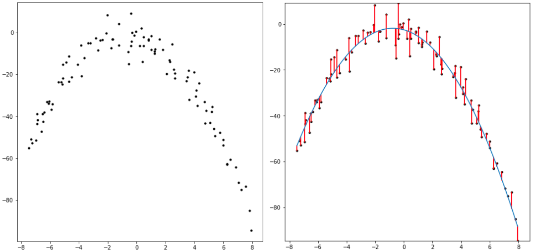
Quadratic regression does the same process as linear regression while adding a third parameter. Instead of optimizing the two variables, slope and intercept, the quadratic regression optimizes three: intercept (p_0), slope when x is zero (p_1), and rate of slope increase (p_2). This is formulated in the equation y = p_2*x^2 + p_1*x + p_0 .

Figure D

Notably, when looking at the equation for quadratic regression, we can see that if the value of p_2 is zero, the equation is the same as the the linear regression. This makes it seem as though the quadratic model is strictly superior to the linear model, since all linear regression results could be reproduced through quadratic regression, obviating the need to ever use the linear regression model. A quadratic model trained on a linear dataset ought to output a linear model, with its quadratic coefficient set to zero. In reality, the addition of an extraneous parameter can harm the model. To see why, it’s helpful to extend this line of reasoning to its logical conclusion.

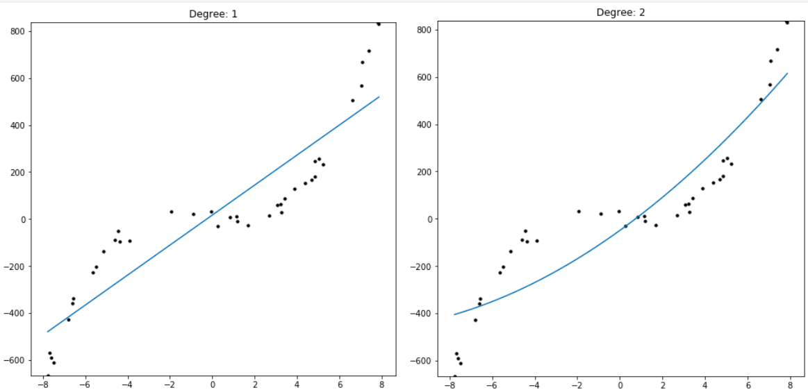
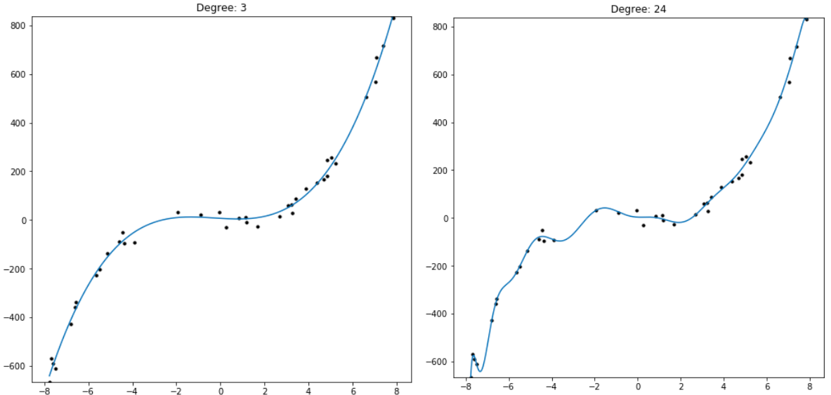
Polynomial regression is a transcendental encapsulation of the pattern formed between average, linear regression, and quadratic regression. Polynomial regression of degree N is regression of N+1 variables over a dataset of (x, y) coordinates: f(x) = p_0 + p_1*x + p_2*x^2 + … + p_N*x^N . A degree one polynomial regression is literally a linear regression. A degree two polynomial regression is a quadratic regression. A degree three polynomial regression is a cubic regression, and so on. This allows us to pick a degree N which corresponds to the complexity of the data we are modeling (Figure E). However, as was the case with quadratic regression versus linear regression, it’s clear from looking at the equation for N degree polynomial regression that a higher degree regression can capture every polynomial regression with a lower degree than it by setting the higher level coefficients. The higher degree polynomials seem to have the capacity to capture all models of lower degree.

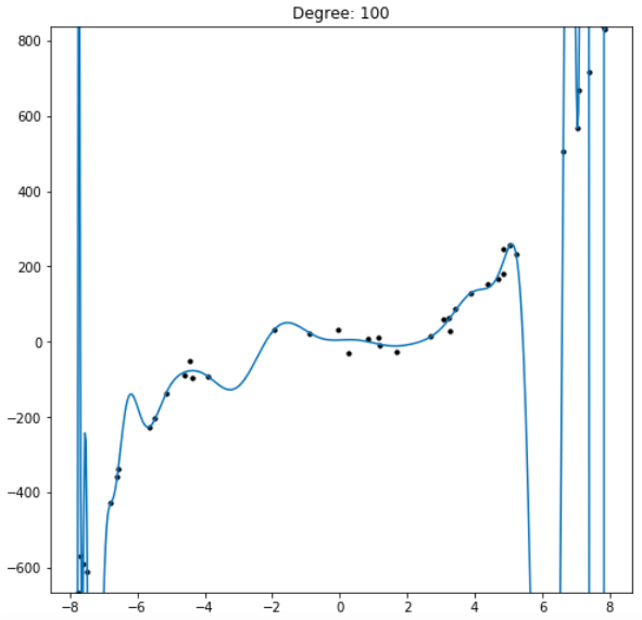
So if a degree 100 polynomial regression has the ability to perfectly describe all regressions 0 through 99 why don’t we use it as default for all our regressions so we don’t have to guess any given dataset’s true underlying degree? Observing the results shows the practical problem with this approach.

Figure E

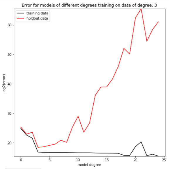
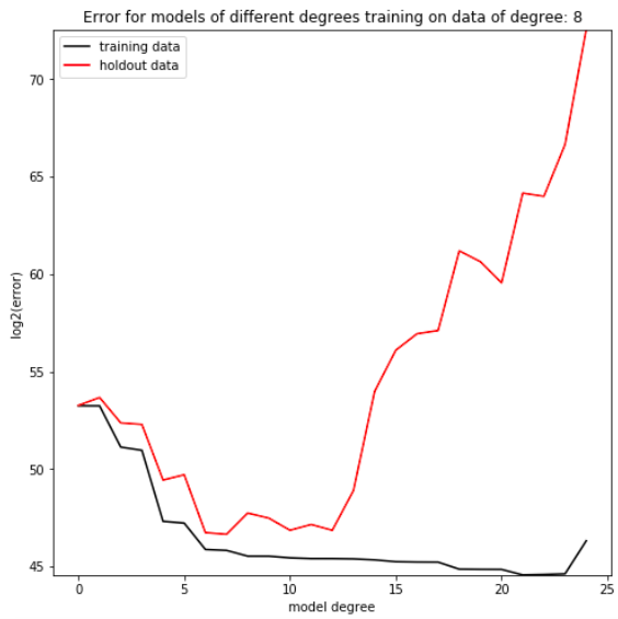
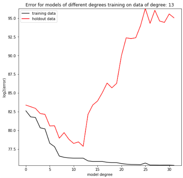
Even though the 100 degree regression can produce a model of a lower degree, in practice it fails to do so. The reason this occurs is that, while the model does minimize the error between its predictions and the given data, it does not capture the data’s overall trend. If we were to find new data from the same distribution as the regression’s training data, the model would be demonstrably worse at predicting that new dataset than a model limited to fewer parameters. By holding out a small proportion of the training dataset and evaluating the trained model on data it hasn’t seen yet, we can simulate this process of testing our model on new data from the same distribution as the training set (Figure F). It’s clear that depending on the complexity of the dataset, there is a degree at which models stop improving, and a degree at which they start getting objectively worse at predicting the holdout data. This phenomenon is called overfitting, in which models which have more freedom than necessary will train on random minutiae in their training dataset, making them worse at capturing the larger patterns in the data. Having a polynomial degree smaller than your data’s underlying degree will yield an insufficient model, but having a polynomial degree far higher than your model’s will yield an overfitted one.

Figure F

Degree is the sole hyperparameter of polynomial regression, in that it determines the number of parameters used in the algorithm instance’s final model: f(x) = p_0 + p_1*x + p_2*x^2+…+p_(degree)*x^(degree). It’s a variable that the programmer of a model chooses. Since there is no clear universally optimal degree, the programmer typically guesses a few reasonable values and analyzes the results of each, repeating the process until they narrow in one a hyperparameter set that works best for a dataset. Guessing and adjusting by hand is a surprisingly time consuming process, especially because it requires the programmer to wait for the model to generate a model, then stop whatever they are doing and analyze the model, often many times for an individual machine learning task. The solution to this problem is to implement a meta-machine learning program to optimize the hyperparameter automatically. This practice is called Hyperparameter Tuning. In the case of polynomial regression, the meta-learning algorithm could pick a low value for the degree, like 0, to start. Then the algorithm would train a model of that degree and evaluate it on holdout data as described above. The algorithm increases the value of degree, re-training and re-evaluating its models until it reaches a local minimum error on the holdout dataset, at which point it returns a model with degree equal to the degree which minimizes the holdout error³. This is the smallest model which. By using a hyperparameter tuning algorithm, every variable described in an algorithm superstructure can be optimized without the need for a programmer to do so by hand.

Part Three: Drawbacks of Hyperparameter Tuning?

While hyperparameter tuning is effective, it is a costly process, with each hyperparameter multiplying the number of models that have to be trained and discarded. In situations where a programmer can analyze what hyperparameters would be most effective without testing them, an unthinking reliance on hyperparameter tuning can increase the time of development⁴. There is no one best solution for how to develop machine learning programs, but hyperparameter tuning is a helpful method in many contexts.

In the pursuit of a complete model for human reasoning, one task which is crucial to the final product is an effective model of reasoning. The ability to combine known facts in order to create new facts is a process humans do effortlessly in our daily lives. When critically applied, the process of producing new facts from existing information helps to forward most, if not every, human endeavor. Modeling this process has, consequently, been attempted and refined many times.

An aside on logical variables and notation:

Propositional Logic Terminology:

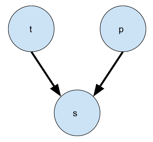
One approach to producing new facts from old ones is binary propositional logic. Propositional logic allows us to capture relations between statements about the world. Say we have three propositions: “the temperature is below 32 degrees” (t), “there is precipitation” (p), and “it is snowing” (s). From these variables we can make a few statements about the relationship between them: “if t and p are true, then s is true” (t ∧ p → s), “if t is false then s is false” (~t → ~s), and “if p is false then s is false” (~p → ~s). These rules let us use limited information we might have to gain more information about the state of the world. Say we know that it’s snowing. From that information and these rules, we can figure out both that it is below 32 degrees and that there is precipitation.

Bayesian reasoning terminology:

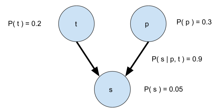
A alternative method for modeling reasoning is Bayesian probability, which, like propositional logic, consists of beliefs and relations between beliefs. The major benefit to bayesian networks over classical logical networks is that, rather than the beliefs and relations being binary, they are probabilistic. This helps immensely, because, outside of the frictionless vacuum that is classical logic, most events and relations between events aren’t known with 100% certainty. Where a classical interpretation of the model above would be easily disprovable with a counterexample (say… hail?), the bayesian interpretation (annotated below) is far more robust.

In dealing with probabilistic events rather than binary facts, Bayesian models capture the incomplete knowledge that we hold about the world. Most statements humans make are collectively understood to be mostly true, but sometimes false. When I say that the bus arrives at 8, nobody would claim I’m a liar if the bus didn’t come one day. My statement clearly isn’t meant to mean that it would be impossible for the bus not to come at 8, but rather that I intend the listener to believe that the bus will arrive at 8. I hold some internal high probability of the bus arriving at 8 (like 99%), and make statements to bring the listener’s probability close to mine. For this reason, taking statements about the world and feeding them into a binary logic machine would in surprisingly often produce unexpected and intractable paradoxes when unlikely scenarios occur that counter the statements programmed into it. By storing probabilities rather than binary facts, the model can recognize when an unlikely but possible event occurs and reason through it.

Even if we did prefer the binary format for facts in terms of communicating information to the person running the inference machine, we could always write rules to convert probabilities into binary facts, whereas we couldn’t do the same in reverse order. We could tell the program to convey knowledge it holds at greater than 95% likely as true, and knowledge it holds at less than 5% likely as false, leaving everything in the middle as so far undecided. That would allow the machine to reason internally with probabilities, but convey knowledge externally as facts. We cannot convert the other way around, because there are only two values in classical logic to project onto a continuous range between probabilities zero and one. If you set every false statement to probability 0 and every true statement to probability 1, you would get a working bayesian network that produces the same results as your binary network, but it would be similarly stuck saying all statements are 100% true or 100% false. Probabilistic models of reasoning are more expressive than binary models in capturing systems of imperfect knowledge.

Next week! The math behind Bayesian reasoning.

Looking at recent advancements in the field of machine learning, it would be hard to ignore neural networks. For the past two decades, neural networks have dominated the field so greatly that individual neural network architectures (patterns of neuron structures) have gone in and out of vogue in that time. Across almost all sub-fields of machine learning, neural networks are now integrated into the core of the endeavor. This phenomenon is especially interesting from a historical perspective, as it wasn’t always the case.

For the majority of machine learning’s history, neural networks were only one of many frequently used techniques, and not always even a top contender. Other data-oriented shallow learning models existed, such as Support Vector Machines and Scale-Invariant Feature Transform, and are still commonly used today, though less so than before the proliferation of neural networks¹. Even less popular now are rule-based methods, which, for a period of time, contended for the future of artificial intelligence. By interrogating how neural networks overtook these competitors, we can gain insight into the conditions necessary for new AI paradigms to arise.

Two factors which ushered in the neural network takeover were (1) a shift in computing power and architecture in the 1990s and 2000s, and (2) an unfilled niche in computer programming that neural networks filled. This should be obvious in retrospect: for any technology to be widely adopted, the technological capacity for its creation (opportunity for development) must exist, and it must perform some task as well or better than alternatives (motive for adoption). A feature of neural networks’ history is that both the opportunity and motive for neural networks cut across a wide band of programming sectors. Because advancements in computing power were not new technologies but rather decreases in existing technologies’ prices², they were available to hobbyists and low-budget developers not long after they became available to large businesses, governments, and research institutions. Their niche, as well, was one general to disparate sub-fields of computing, which made neural networks useful to implement for vastly different endeavors.

The first half of neural networks’ opportunity for adoption dawned in the 1990s, as the continual advancement of computing power reached a point where training a multilayer network was feasible. As years went on, it took less and less time to train iterative learning models on a traditional CPU, allowing for an unprecedented rapid development of those machine learning techniques. In the mid-2000s, graphics processing units (GPUs) became inexpensive as supply rose to meet the demand from computer graphics (primarily 3D modeling and video games). Programmable GPUs are physically structured differently from traditional CPUs, and allow for incredibly efficient parallel processing, so their proliferation caused a discrete leap in the efficiency of all parallelizable programs, neural networks included. This combination of factors sets the stage for neural networks’ consideration as a viable method of everyday machine learning.

Of course, a technology’s computational viability couldn’t be the sole determiner of its popularity. There’s a historic paradox in computer programming relevant to the niche neural networks fill: tasks which humans need to be taught are generally easy to encode into computers, while tasks which come innately to humans are historically difficult to encode. Humans naturally acquire sight, but it took until the 21st century for computer programs to to parse complex images at a usable level, whereas humans need to be taught arithmetic over many years, a skill which was one of the earliest encoded into computers. Somehow the things we find easiest to do are the hardest to convey to computers. This paradox is the consequence of the fact that humans are not consciously aware of the steps involved in executing the tasks which our brains execute frequently and efficiently. We don’t intuitively know how our eyes convert photons into visual objects. We don’t intuitively know how we process language. We only have awareness of these processes inputs and outputs, not their internal workings. Attempts to encode these tasks traditionally evade simple eloquent solutions³. Even through intense prolonged introspection, we haven’t been able to fully decode these black box mechanisms in our own minds. One explanation for this is that these tasks are not computed in our brains using rigorous algorithms, but rather messy associative structures of neurons ⁴, ⁵. This “messy structures hypothesis” is supported by the recent solutions to these seemingly unencodable problems. Deep neural networks, in training broad structures of neurons on large input datasets, have revolutionized fields that involve mimicking unconscious thought, like Computer Vision, Natural Language Processing, and Data Classification. In mimicking unconscious thought’s characteristics, Neural Networks are better at mimicking their function than any prior technology. With the availability of neural networks programmers could finally automate tasks that once required a human’s unconscious to complete.

With the understanding of how neural networks came to dominate machine learning, we can also understand why their competitors fell to the wayside. Shallow learning models are still used to this day, as they have the benefit of generally being faster to implement and more reliable than machine learning methods with less training time. No, as stated above, other than the rise in Neural Networks, the most striking difference in the Artificial Intelligence field between the 1990s and now is the fall of rule-based methods. Rule-based methods learn by constructing patterns of rules formatted from atoms. They were a popular area of research in the late 20th century, and encompassed Expert Systems, which were pre-programmed rule-sets used to encode and distribute automated expertise. Rule-based methods displayed promise, but didn’t seize the zeitgeist when computing power developed. While neural networks filled a desperately lacking niche in the field, rule-based methods automated logical analysis and knowledge encoding, two tasks that programmers are trained to perform efficiently. While the technological opportunity for their advancement was increasing, the motive decreased in relation to its alternatives. In this feedback loop, rule-based methods were put on the field’s back-burner, to the point that they are unknown now to many programmers.

This analysis of opportunity and motive not only explains the past, but can predict the future of Artificial Intelligence. We already see a niche forming in the gaps left unfulfilled by neural networks. As the intractable problems of transparency and modularity become more apparent, we will likely see a machine learning paradigm which is more adept at those tasks increase in funding and interest.

Most of reality is comprised of continua, or attributes which vary continuously between possible values. Examples could be distance, weight, age, or confidence. Constructs which humans create, on the other hand, are discrete, meaning they exist in categories. Discrete corollaries to the previous examples are far versus near, heavy versus light, old versus young, and confident versus unconfident. One hypothesis as to why we think this way is that, to analyze a phenomenon, it’s easier to reason about things which fall under a category (a binary inclusion or exclusion of any datapoint) than things which fall on a continuum. We can look at objects which are heavy and observe that all of these fall at the same rate, while light things, like feathers, sometimes fall slower, even though we on some level recognize that light and heavy are discontinuous constructs we created over a continuous underlying reality. It’s also easy to observe from after the fact that the theory over constructs is less accurate than the theory over continua, i.e. that we can calculate the force of drag in relation to the force of gravity on any object given its weight and shape, and use that to determine its rate of acceleration. However, without the discontinuous theory, it would be hard if not impossible to develop the continuous theory, as the continuous theory would have to be created out of whole cloth with no logical or observational intermediates—a kind of analytic immaculate conception. So we play out this charade in developing discrete theories, where we find a concrete observation (things at this section of the spectrum perform this way, and things at this section perform that way), with the common knowledge that that is likely the product of some underlying function over a continuum. Then, once our discrete theory is validated, we extend it into the space which better represents reality. This Discrete Charade must be properly understood as a valuable step in the development of new theories, with the common understanding that this scaffolding will likely be obsoleted later by a more precise continuous model.

Note: A general familiarity with multiple machine learning methods is assumed here. Understanding on a broad level how neural networks¹, decision trees², and linear regression³ work should be sufficient to understand the content.

When explaining machine learning methods, analogies to the human mind can prompt intuition for what part of human cognition the learning method is re-creating. On the broadest level these analogies are words like “learning,” and “training,” which describe processes general to arguably all machine learning methods ⁴. More thoroughly defined sub-fields of machine learning are described with increasingly specific analogies. Supervised and unsupervised learning, for example, describe different methods of pedagogy shared between humans and two types of machine learning algorithms. This process of iterative specification continues to the point of specifying an individual algorithm’s form and function.

Certain neural network structures are described with these metaphors, which helps people learning about them determine those structures’ use cases. In the space of recurrent neural network structures, processes like “attention,” (transformers) and “short-term memory,” (LSTMs) provide insight into the intended and expected features of those networks. Generative Adversarial Networks are another type of neural network, named as such because they train by pitting two antagonistic networks against each other. Having an idea of what a network is doing on a high level— understanding what about them is similar to the human epistemic process—makes it much easier to judge their efficacy and understand their limitations.

While analogies between specific neural network structures and the human mind exist, on of scope of neural network architecture as a whole, comparisons are usually to the mind on a materialistic level, e.g. computational neurons are compared to human neurons (though that isn’t very accurate ⁵). It’s rare to see explanations of what thought processes deep neural networks imitate for what seems like a good reason: the lack of pre-defined structure in the sub-field of neural networks appears to allow different types of them to train towards any solution necessary. What would it mean to describe an architecture that is so flexible and universal? While this blank-slate argument appears to end the discussion on neural network-human mind analogues, it can serve to obscure the subjective reality of neural networks.

Grant Sanderson, in his video “But what is a neural network?”, described how one might expect the first layer of a neural network training on the MNIST dataset to identify lines and dots, then the second to identify intersections and primitive shapes from the prior layer’s output, and the third to compose shapes into more complicated structures, but, when the network finishes training, in actuality the layers’ contents are a mess. This is true of almost all neural network architectures which don’t heavily rely on very specific directions from the programmer—the internal contents of neural networks are unintelligible by consequence of their inherent structure. As neural networks update their internal weights and biases, there is no value associated with intelligibility, which demonstrably results in their disorganization.

One explanation for the lack of subjective cognitive analogies here is a distinct difference between neural networks and other types of machine learning. Most other types of machine learning model a task we can perform consciously, or at least on command. Clustering 2D and 3D data is a stunningly easy task for humans. Polynomial regression is a conscious process we learn to perform in algebra and statistics. Creating decision trees is a task for storing information so common there are jokes about their overuse (https://xkcd.com/518/). Iterative backpropagation on the other hand… isn’t so easy. Unlike other methods, there isn’t a conscious way to invoke the human analogue to deep neural networks, even though they’re based on our neurons…

When I look around my room, I see my shoes, a computer, some pillows, a desk. This I understand effortlessly, and comes without the need to reason through the steps from raw visual data to a conceptual object. I can attempt to reproduce my thought process, focusing on the parts of the shoe that my eye used to assess its shoe-ness, but I have no way to verify that analysis’s accuracy; it’s purely speculation. The outputs of our visual processing are intuitively available to the seer. With effort, the seer can become aware of the raw inputs to their visual process, but the steps in between input and recognition are consistently a mystery. This mirrors the conceptual structure of neural networks surprisingly well, with messy inputs, a clear output, and an inscrutable process between the two.

Logical analogue for deep classification NNs This analysis can be extended to logical reasoning. Neural networks that map from large feature sets to a set of outputs have the same pattern of clarity as the visual neural networks described above, but serve the function of categorizing the data into relevant concepts. When we perform patterns of thought frequently enough, our brains create heuristics to make those patterns faster. Walk outside just before a rainstorm, and notice how you can tell it’s going to rain even before you choose to evaluate why you know that. Watch your dog start to salivate at the sound of the dinner bell. These black-box associative processes are very powerful, and incredibly fast once trained⁶.

With the power of associative learning methods in mind, it’s important to understand their limitations. Because they have no structural intermediates, they can be subject to invisible bias, where certain combinations of inputs which were biased in the sample set are transferred to the final model without anyone knowing. They also don’t have the inherent structural capability to simplify and convey their conclusions to a human or other machine learning structure. One method of human reasoning is the establishment of facts upon evidence and higher order facts upon other facts. Neural networks, in having fixed complexity⁷ and no way to fix a useful set of neurons (analogous to a lemma here) in place, are not structurally designed to perform this task, and so will only arrive at reusable logical intermediates to their conclusions on chance. Unconscious learning models certainly have a place in artificial intelligence, but are structurally inadequate to model conscious thought processes. Some problems are simply not suited for neural networks.