Part One: What are Hyperparameters?

Figure A

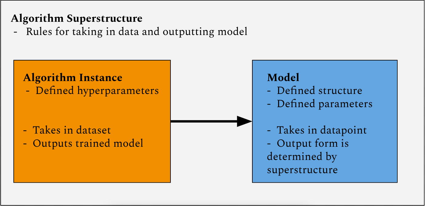
The term ‘machine learning algorithm’ is ambiguous. The component of machine learning that the public interacts with most frequently is the machine learning model, which takes data and processes it to produce an actionable result. The youtube recommendation algorithm is a machine learning model which takes in data about a user as well as data about videos on the site and recommends the user videos that optimize for sustained watch-time. Programmers are introduced to machine learning from the other end. Computer science courses introduce students first to machine learning algorithm superstructures: the steps for generating and optimizing the parameters of a model. Each algorithm superstructure also defines the format of its model, i.e. what its inputs, outputs, and intermediate structures can look like. Typically a machine learning algorithm superstructure provides some amount of flexibility in its output model structure. Between the two is the algorithm instance, which is an individual invocation of the superstructure with a set of hyperparameters that define a rigid form for the model’s structure within the broader space allowed by the superstructure. The instance is executed on a computer and trains its model’s parameters to be optimal over a provided training dataset. If a given machine learning model is a bicycle, the algorithm instance which produces it is the bicycle factory which produced it, and the model superstructure is a design document for factories that produce bicycles.

Hyperparameters exist at an interesting location within this taxonomy, because while choosing the right values for them is very important to generating an effective model for a given dataset, they cannot be adjusted during the model training process, since they determine the shape of the model. They must be defined before the expensive training process is executed.

Part Two: A Case Study in Hyperparameters

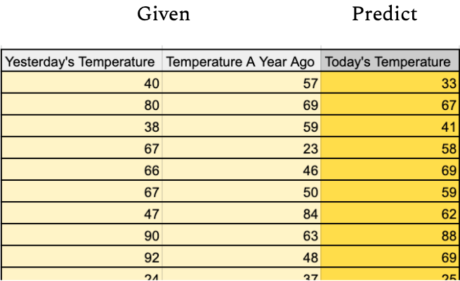
Regression algorithms are a subset of machine learning algorithm superstructures which, given a set of input values and their corresponding output values, generates a model to map those inputs to their outputs¹ (Figure B). Figure B

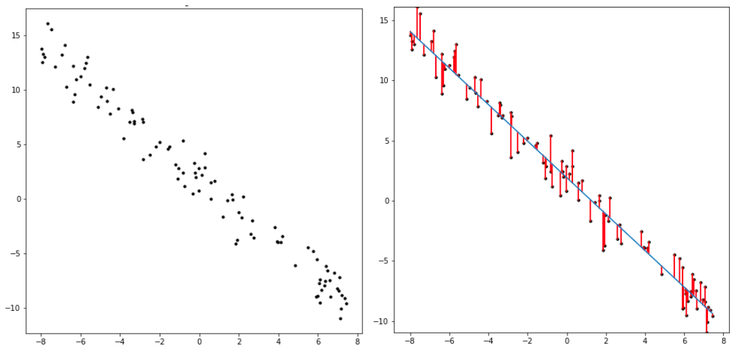
Linear regression is a simple example of this type of algorithm. It generates a line² that most closely fits a set of datapoints. The way it measures closeness between the line and the dataset is the difference between the line’s predicted y value (f(x)) for a given datapoint’s x coordinate, and the datapoint’s actual y coordinate. It optimizes two parameters: the x-intercept of the line (p_0) and the line’s slope (p_1), which are used in the relation defining the line: f(x) = p_1*x + p_0 . The linear regression algorithm finds the values of p_0 and p_1 which minimize the difference between f(x) and y for all (x, y) datapoints provided.

Figure C

Quadratic regression does the same process as linear regression while adding a third parameter. Instead of optimizing the two variables, slope and intercept, the quadratic regression optimizes three: intercept (p_0), slope when x is zero (p_1), and rate of slope increase (p_2). This is formulated in the equation y = p_2*x^2 + p_1*x + p_0 .

Figure D

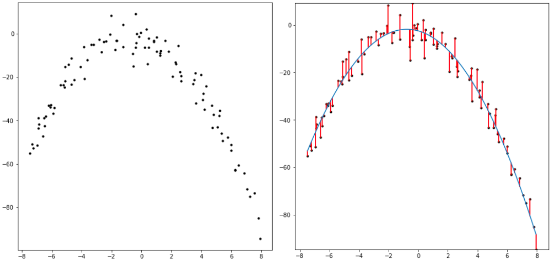
Notably, when looking at the equation for quadratic regression, we can see that if the value of p_2 is zero, the equation is the same as the the linear regression. This makes it seem as though the quadratic model is strictly superior to the linear model, since all linear regression results could be reproduced through quadratic regression, obviating the need to ever use the linear regression model. A quadratic model trained on a linear dataset ought to output a linear model, with its quadratic coefficient set to zero. In reality, the addition of an extraneous parameter can harm the model. To see why, it’s helpful to extend this line of reasoning to its logical conclusion.

Polynomial regression is a transcendental encapsulation of the pattern formed between average, linear regression, and quadratic regression. Polynomial regression of degree N is regression of N+1 variables over a dataset of (x, y) coordinates: f(x) = p_0 + p_1*x + p_2*x^2 + … + p_N*x^N . A degree one polynomial regression is literally a linear regression. A degree two polynomial regression is a quadratic regression. A degree three polynomial regression is a cubic regression, and so on. This allows us to pick a degree N which corresponds to the complexity of the data we are modeling (Figure E). However, as was the case with quadratic regression versus linear regression, it’s clear from looking at the equation for N degree polynomial regression that a higher degree regression can capture every polynomial regression with a lower degree than it by setting the higher level coefficients. The higher degree polynomials seem to have the capacity to capture all models of lower degree.

So if a degree 100 polynomial regression has the ability to perfectly describe all regressions 0 through 99 why don’t we use it as default for all our regressions so we don’t have to guess any given dataset’s true underlying degree? Observing the results shows the practical problem with this approach.

Figure E

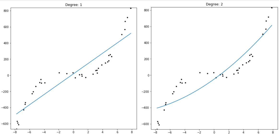
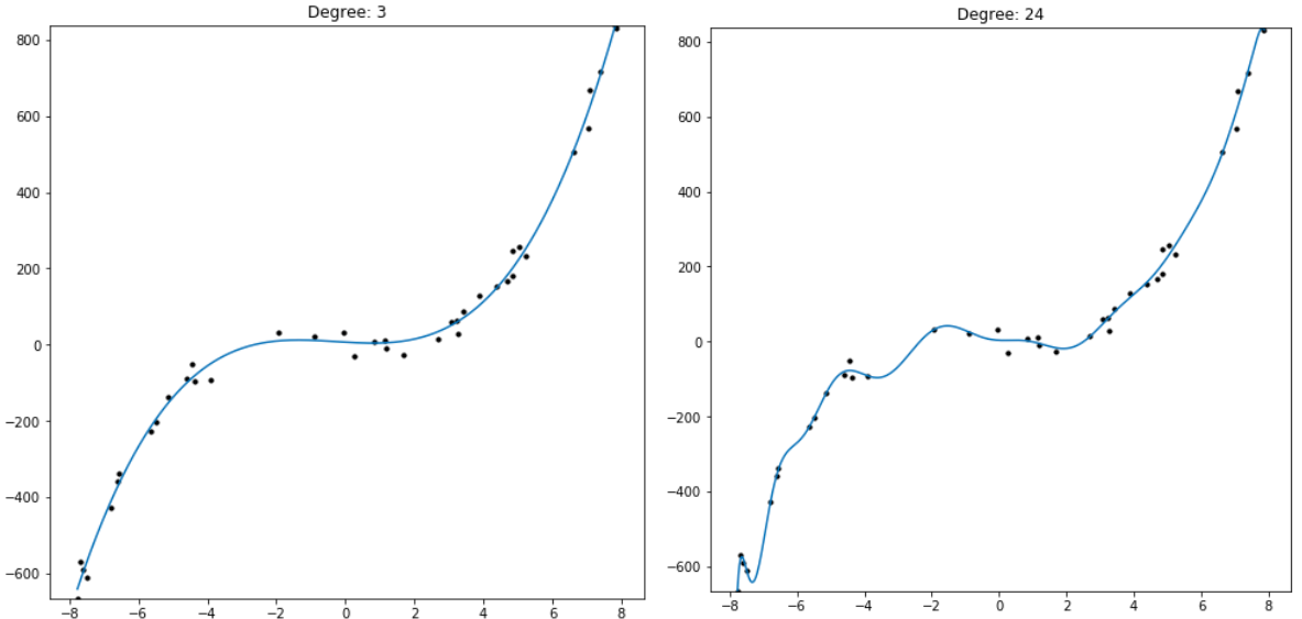
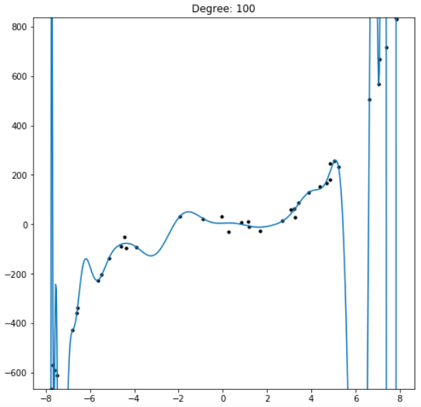
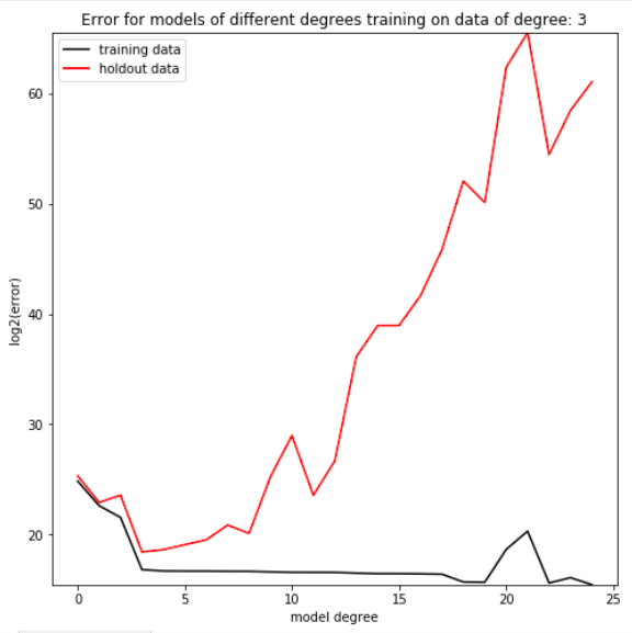
Even though the 100 degree regression can produce a model of a lower degree, in practice it fails to do so. The reason this occurs is that, while the model does minimize the error between its predictions and the given data, it does not capture the data’s overall trend. If we were to find new data from the same distribution as the regression’s training data, the model would be demonstrably worse at predicting that new dataset than a model limited to fewer parameters. By holding out a small proportion of the training dataset and evaluating the trained model on data it hasn’t seen yet, we can simulate this process of testing our model on new data from the same distribution as the training set (Figure F). It’s clear that depending on the complexity of the dataset, there is a degree at which models stop improving, and a degree at which they start getting objectively worse at predicting the holdout data. This phenomenon is called overfitting, in which models which have more freedom than necessary will train on random minutiae in their training dataset, making them worse at capturing the larger patterns in the data. Having a polynomial degree smaller than your data’s underlying degree will yield an insufficient model, but having a polynomial degree far higher than your model’s will yield an overfitted one.

Figure F

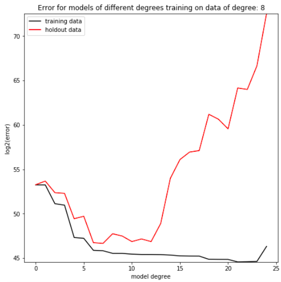
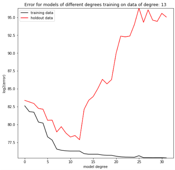
Degree is the sole hyperparameter of polynomial regression, in that it determines the number of parameters used in the algorithm instance’s final model: f(x) = p_0 + p_1*x + p_2*x^2+…+p_(degree)*x^(degree). It’s a variable that the programmer of a model chooses. Since there is no clear universally optimal degree, the programmer typically guesses a few reasonable values and analyzes the results of each, repeating the process until they narrow in one a hyperparameter set that works best for a dataset. Guessing and adjusting by hand is a surprisingly time consuming process, especially because it requires the programmer to wait for the model to generate a model, then stop whatever they are doing and analyze the model, often many times for an individual machine learning task. The solution to this problem is to implement a meta-machine learning program to optimize the hyperparameter automatically. This practice is called Hyperparameter Tuning. In the case of polynomial regression, the meta-learning algorithm could pick a low value for the degree, like 0, to start. Then the algorithm would train a model of that degree and evaluate it on holdout data as described above. The algorithm increases the value of degree, re-training and re-evaluating its models until it reaches a local minimum error on the holdout dataset, at which point it returns a model with degree equal to the degree which minimizes the holdout error³. This is the smallest model which. By using a hyperparameter tuning algorithm, every variable described in an algorithm superstructure can be optimized without the need for a programmer to do so by hand.

Part Three: Drawbacks of Hyperparameter Tuning?

While hyperparameter tuning is effective, it is a costly process, with each hyperparameter multiplying the number of models that have to be trained and discarded. In situations where a programmer can analyze what hyperparameters would be most effective without testing them, an unthinking reliance on hyperparameter tuning can increase the time of development⁴. There is no one best solution for how to develop machine learning programs, but hyperparameter tuning is a helpful method in many contexts.